
Compute & Silicon
Why a Cold Cache Changes the Meaning of a Fast Response Test
A service that has recently handled a request may respond differently from one meeting it for the first time. Data, compiled work or model state can already be available, so a warm test and a cold test answer different questions.


Photo: Kevin Ache / Unsplash
A service that has recently handled a request may respond differently from one meeting it for the first time. Data, compiled work or model state can already be available, so a warm test and a cold test answer different questions.
The operating distinction
Caches keep selected information close to where it will be used. Reusing that information can reduce retrieval or preparation work. A cold start may need to rebuild it, load a model or fetch data from a slower location. Neither condition is inherently the only valid test; the expected workload determines the mix.
Preparation can also occur outside the part of the system being timed. A demonstration may load information before starting its stopwatch, while a user experiences that loading as part of the wait. That does not invalidate the demonstration, but it changes the boundary of the claim.
A practical example
Imagine comparing two demonstrations of the same service. One repeats a familiar query while the other begins after a restart. Their response times may differ without any change in the underlying hardware. A fair comparison describes what was already loaded and what preparation was included.
Questions worth asking
A comparison should include preparation that matters to the intended user experience. Keeping warm and cold observations separate makes both useful without presenting the faster result as representative of every possible request.
- Was the test performed after restart or after repeated requests?
- Which preparation steps were included in the measured response?
- How often does the real workload encounter the cold condition?
What the evidence supports
A single fast example cannot establish the experience across restarts, uncommon requests and traffic changes. Conversely, an unusually slow first request should not automatically represent steady operation. Readers need the operating state, the sampling method and the service objective before drawing a conclusion.
A useful comparison can present both first-use and repeated-use observations under clearly described conditions. It should identify whether the test reuses the same request or exercises a broader set of inputs. The reader can then decide which observation resembles the intended application. The aim is an honest description of service behavior, not a contest that rewards whichever test omits the most preparation work.
Treat cache state as part of the test description, alongside the machine and the application.
Quick check
How much did you catch? Tap a question to see the answer.
1. Why do warm and cold tests give different results?
Answer: Data, compiled work or model state may already be loaded in a warm test.
2. Is a cold test the only valid one?
Answer: No. The expected workload decides the right mix.
3. What should a fair comparison describe?
Answer: What was already loaded and what preparation was included in the timing.
Where Warm State Lives in a Modern Service
The word cache can sound like a single component, but a typical service holds several layers of prepared state at once. Each layer can be warm or cold independently, which is one reason response tests can be difficult to compare.
- Model weights in memory. A model already loaded onto an accelerator is ready to run. A model that must be read from storage first adds loading time.
- Compiled or optimized code. Some systems prepare optimized execution paths the first time a particular shape of work appears and reuse them afterward.
- Request-level reuse. Inference systems may reuse computation for repeated prompt prefixes or recently seen inputs.
- Application data caches. Frequently retrieved documents, records or results may be held in faster memory near the service.
- Connection and session state. Established network connections, authentication tokens and open sessions avoid setup work for subsequent requests.
- Storage and operating system caches. Files read recently may already sit in memory, making later reads faster.
Designing a Fairer Response Test
Anyone evaluating a claim about response speed, or designing a test of their own, can work through a short sequence.
- Describe the starting state. State whether the test began after a restart, after a period of inactivity or after a run of similar requests.
- Define the timing boundary. Record exactly when the clock starts and stops, and which preparation steps fall inside or outside that window.
- Vary the inputs. Use a set of requests that resembles the real workload rather than repeating one query.
- Report a distribution. Present typical and slower responses, not only the fastest or the average.
- Estimate the real cold rate. Consider how often actual users will meet a cold condition, based on traffic patterns, scaling behavior and restarts.
- Keep the results labeled. Publish warm and cold observations side by side with their conditions.
Common mistakes
A frequent mistake is running a test many times and reporting the best result, which almost always reflects fully warm conditions. Another is forgetting that automatic scaling can introduce cold starts whenever new capacity is added during a traffic increase. A third is comparing two systems where one test included model loading and the other did not. A fourth is assuming that a cold start happens only after a deliberate restart, when cache eviction under memory pressure can produce similar effects.
What This Means for Buyers and Readers
For a business choosing an inference service or reading a vendor’s performance claim, the cache question is practical. A service that is consistently fast for repeated requests may still feel slow to users who arrive with varied or uncommon requests, or who arrive just after a scaling event. Asking how the provider handles cold conditions, and how often they occur in practice, gives a more realistic sense of what users will experience.
Fast is a description of a particular state. The useful question is how often the real workload is in that state.
Questions Readers Ask
Is a warm test misleading?
Not if it is labeled. Warm results describe steady operation for repeated work, which is useful. They become misleading only when presented as the whole experience.
Can cold starts be eliminated?
They can be reduced by keeping capacity loaded and preparing state in advance, but this usually carries a cost in reserved resources.
Why does the first request after a restart take longer?
The service may need to load models, prepare execution paths, open connections and fill caches before it can respond.
What should a buyer ask a provider?
Ask what conditions their published response figures assume and how the service behaves after restarts, scaling events and long idle periods.
AI infrastructure explainers and news on iPhone, iPad and Apple Watch.
Latest stories
View all


Compute & Silicon
An Idle Accelerator Can Still Be Waiting on Useful Work
A low utilization reading does not identify a single problem. An accelerator can be waiting for data, another machine, a scheduling decision or a request from a user. Understanding the waiting state matters more than assigning blame to the chip.
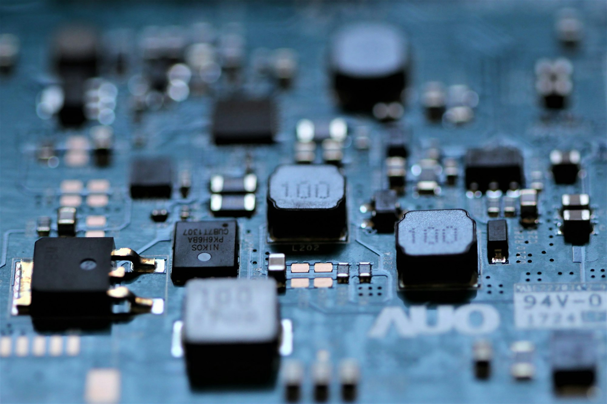
Photo: Anne Nygård / Unsplash
A low utilization reading does not identify a single problem. An accelerator can be waiting for data, another machine, a scheduling decision or a request from a user. Understanding the waiting state matters more than assigning blame to the chip.
The operating distinction
Useful work passes through several stages before an accelerator starts arithmetic. Data must be available, memory must have room and dependent tasks must finish. A scheduler may also hold capacity for a workload with a deadline. That reserved headroom can look similar to inefficiency on a broad average.
Different kinds of waiting call for different responses. Adding processors will not necessarily repair a slow input pipeline, and changing scheduling can affect one customer's response while improving another's throughput. The resource graph and the service objective need to be read together.
A practical example
Imagine an inference service that keeps spare resources available for sudden requests. Filling every available slot with background work could increase the average utilization while making urgent requests slower. A training job with predictable input and long execution periods would present a different operating problem.
Questions worth asking
Reserved headroom, missing input and inefficient execution are different explanations for unused capacity. The next operational question should follow the observed cause rather than assume that every idle interval represents the same problem.
- What resource or dependency is the accelerator waiting for?
- Does the measurement include reserved capacity and maintenance periods?
- Did higher utilization improve completed work or merely lengthen queues?
What the evidence supports
Utilization needs a definition and a time window. A device-level percentage alone cannot show whether a service met its response target or whether a job completed on schedule. Compare the waiting causes and user outcome before comparing the headline averages.
A useful account identifies the interval when the observation was made and describes the mix of jobs present. Readers can then distinguish an idle system with no demand from a busy service deliberately retaining headroom. Both can show unused device capacity, but they tell different stories about the amount of work waiting and whether customers are receiving the experience the service was designed to provide.
The useful target is productive work within the service requirement, not a percentage detached from its purpose.
Quick check
How much did you catch? Tap a question to see the answer.
1. Does low utilization point to a single problem?
Answer: No. An accelerator may be waiting on data, another machine, scheduling or users.
2. Why can reserved headroom look inefficient?
Answer: It can resemble idle capacity on a broad average.
3. Will adding processors fix a slow input pipeline?
Answer: Not necessarily.
Sorting Idle Time Into Categories
A single utilization line becomes far more useful once the unused intervals are split into a few named categories. The categories do not need to be elaborate. They only need to separate explanations that call for different responses, so that a review meeting can discuss causes instead of a number.
- No demand. Nothing was waiting. The service was available and nobody needed it during that interval.
- Deliberate headroom. Capacity was held back on purpose so urgent or latency-sensitive requests could start quickly.
- Input starvation. Work existed, but data, model weights or request batches were not arriving fast enough to keep the device busy.
- Coordination waits. The device was ready but waiting on another machine, a synchronization step or a dependent task.
- Scheduling gaps. Work was queued, yet placement, priority or fragmentation kept it from landing on available hardware.
- Planned unavailability. Maintenance, testing, updates or recovery activity removed the device from service.
Even a rough split changes the conversation. If most idle time belongs to deliberate headroom, the question becomes whether the reserve is sized correctly for the response target. If most belongs to input starvation, the attention moves to storage, networking or preprocessing. Neither answer requires buying or removing accelerators.
A Step-by-Step Review of Unused Capacity
An operator or analyst trying to understand a low reading can work through a short sequence before drawing conclusions.
- Fix the time window. State whether the figure covers an hour, a day, a month or a reporting quarter. Overnight lulls and weekend demand can dominate a long average.
- State what counts as busy. Some measurements record whether any work is scheduled on the device, while others try to estimate how much of its arithmetic capability is in use. The two can tell very different stories.
- Separate the workload mix. Training, batch processing and interactive inference have different shapes. Averaging them together hides the behavior of each.
- Place the waits on a timeline. Line up idle intervals against data transfers, checkpoint writes, job starts and request bursts. Patterns often appear where they would never show in a single percentage.
- Check the outcome. Ask whether jobs finished on schedule and whether response targets were met during the same window.
- Choose the response that matches the cause. Only then decide whether the answer is more capacity, better scheduling, a faster input path or no change at all.
Common mistakes
The most frequent error is treating utilization as a goal in itself. A team rewarded for a higher figure can fill reserved headroom with low-priority work, which raises the average while making urgent requests wait. Another mistake is comparing utilization across facilities or providers without confirming that the definitions match. A third is ignoring the cost of reaching a higher number, such as longer queues or more frequent preemption of jobs that then have to restart.
What This Means for Readers Following the Industry
Utilization figures appear in earnings discussions, vendor presentations and infrastructure announcements. For a reader trying to understand the business, the figure is a starting point for questions rather than a verdict. A high number may reflect strong demand, or it may reflect a fleet with too little headroom for spikes. A low number may signal weak demand, or a service that keeps capacity in reserve because its customers expect fast responses.
The more useful question is usually what the figure was designed to show and what it leaves out.
This is general education about how infrastructure metrics are read, not a view on any company or security. Anyone weighing a financial decision should consult a qualified financial professional about their own situation.
Questions Readers Ask
Is a fully utilized accelerator always the efficient outcome?
Not necessarily. A device kept constantly busy may leave nothing available for sudden requests. Whether that is efficient depends on the service the device is meant to support.
Can idle time be measured precisely?
It can be measured, but the result depends on the definition, the sampling interval and the tools used. Short waits can disappear inside coarse samples.
Why would a provider intentionally leave capacity unused?
To meet response commitments, absorb failures, allow maintenance or accept new work without delay. Each of those purposes has value that an average cannot display.
What is the single best follow-up question?
Ask what the accelerator was waiting for during the idle intervals. The answer points toward the next useful decision.
AI infrastructure explainers and news on iPhone, iPad and Apple Watch.
Compute & Silicon
Custom AI ASICs vs. GPUs
Custom AI ASICs can deliver strong efficiency on a narrow workload, while GPUs remain valuable because their software ecosystem and flexibility absorb uncertainty.

The custom-ASIC-versus-GPU debate is often framed as a contest between a cheaper chip and a more expensive one. That misses the real decision. A GPU is a general-purpose accelerator with a large software ecosystem. An application-specific integrated circuit is a narrower machine designed around a workload, a power target, or a system architecture.
The winner depends on whether the workload is stable enough to justify specialization. Training, inference, recommendation, search, and video pipelines do not stress hardware in exactly the same way. A model that is efficient today can change after a new architecture, quantization method, context length, or customer demand appears.
What the GPU buys
A GPU’s first advantage is optionality. It can run different model families, numerical formats, kernels, and frameworks. It can be reassigned when demand shifts. That matters for a cloud provider serving many customers and for a company whose AI roadmap is still moving.
The second advantage is software. Mature compiler tools, libraries, kernels, orchestration systems, and developer familiarity reduce the risk between purchasing hardware and putting it into production. A GPU’s list price is not the whole cost; neither is an ASIC’s lower unit cost if engineers spend months rewriting software.
The third advantage is scale. GPUs can be linked into standard or proprietary fabrics, with established server, cooling, and support ecosystems. A customer can often rent them before it owns them, which converts a large capital decision into a more flexible operating expense.
The GPU’s weaknesses are also clear. The chip may carry circuitry for workloads the customer does not use. Its memory and network design may be optimized for a broad market rather than one application. High demand can create shortages, and power density can push a facility’s cooling and electrical systems beyond their original design.
What the ASIC buys
A custom ASIC can remove general-purpose features and use the saved area or power for the specific operations that matter. It may deliver more performance per watt, better latency, or lower cost per inference when the workload is predictable.
An ASIC can also be part of a broader system strategy. Google and other hyperscalers have built custom accelerators because owning the silicon roadmap can reduce dependence on a merchant vendor and let the company tune hardware to its software stack. Intel described an expanded 2026 collaboration with Google around custom ASIC-based infrastructure processing units that offload networking, storage, and security functions from host CPUs. That is a reminder that “custom AI silicon” is not limited to a chip that performs matrix multiplication.
The costs appear before production
ASIC design requires architecture, verification, physical design, software, packaging, testing, and manufacturing commitments. A company must pay those costs before it knows how many units it will ship.
The minimum efficient volume can be high. If a custom chip saves $1,000 per accelerator but costs $300 million to develop and qualify, the business needs more than 300,000 units before ignoring financing, support, and inventory risk. If the workload changes before that volume is reached, the savings may disappear.
Advanced packaging and high-bandwidth memory can add another constraint. Micron reported in March 2025 that its HBM output for calendar 2025 was sold out and that it was already discussing 2026 demand with customers. A custom ASIC that cannot secure memory, substrates, and packaging is not a complete product.
A practical comparison must use system metrics
Compare the two options at the system level. Measure useful work per rack, tokens per second per watt, cost per million tokens, time to train, memory capacity, software migration effort, and failure-recovery behavior.
Do not compare a peak chip number from a data sheet with a measured production result from another platform. Ask whether the benchmark uses the same model, batch size, sequence length, precision, compiler version, and utilization target.
A GPU may win on time to market even if an ASIC wins on energy. The value of six months of earlier service can be material for a cloud provider. Conversely, an inference fleet with a stable model and high utilization may benefit from a specialized accelerator.
The market is moving toward heterogeneous systems
The likely outcome is not one winner. General-purpose GPUs will remain useful for training, new models, and workloads with uncertain demand. Custom ASICs will take more of the predictable inference, networking, storage, and recommendation work. CPUs, DPUs, and specialized accelerators will handle other parts of the system.
Intel’s Gaudi 3 product materials emphasize standard Ethernet, open software, and a migration path for customers moving from GPU-based systems. That positioning shows the market’s pressure point: customers want acceleration without locking every layer of the stack to one vendor.
The decision rule is simple. Use GPUs when flexibility, software, and deployment speed are worth paying for. Use an ASIC when the workload is stable, volume is large, memory and packaging are secured, and the organization can support a separate software and operations path.
The best analysis treats silicon as a fleet decision, not a chip-shopping exercise. The question is which architecture produces reliable, adaptable work at the lowest total cost over the period in which the workload is likely to remain stable.
There is also a strategic lock-in cost. A GPU fleet may be portable across cloud providers and model frameworks, while a custom accelerator can require a dedicated compiler, kernel library, scheduler, and support team. That lock-in may be acceptable when demand is large and stable. It is dangerous when the business case assumes a model architecture will remain unchanged for five years. The best ASIC programs preserve a fallback path: compatible APIs, exportable model formats, or enough GPU capacity to absorb new workloads while the specialized stack catches up.
Sources
- Micron, “Fiscal Q2 2025 Investor Materials,” March 20, 2025: investors.micron.com
- TSMC, “2025 Annual Report,” 2026: investor.tsmc.com
- Intel, “Intel Gaudi AI Accelerator Products,” accessed October 2026: intel.com
- Intel, “Intel and Google Deepen Collaboration to Advance AI Infrastructure,” April 9, 2026: newsroom.intel.com
- IEA, “Energy and AI,” April 10, 2025: iea.org
BOSSTOX Research articles are drafted with AI assistance and reviewed by our editors before publication. See our editorial standards.
Compute & Silicon
HBM Is a Bottleneck Because AI Memory Is a Stack, Not a Chip
High-bandwidth memory limits AI accelerator shipments through several linked manufacturing steps, so a strong DRAM market alone does not guarantee enough HBM for the next GPU cycle.
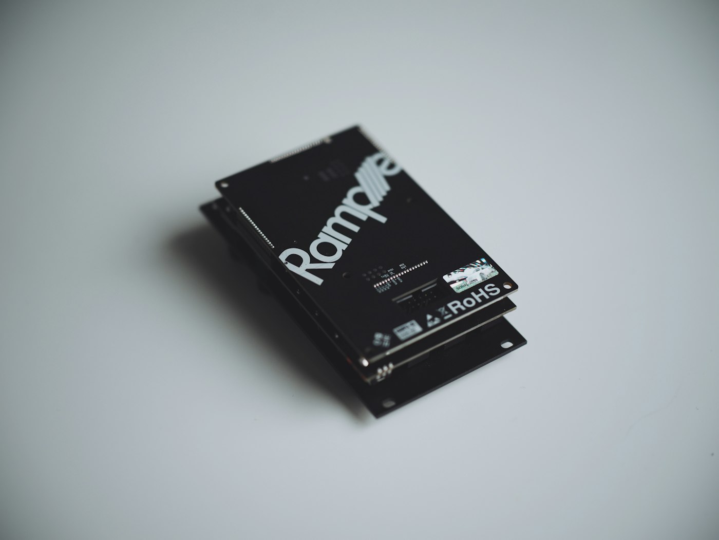
The memory next to the compute
High-bandwidth memory, or HBM, is the memory placed close to an AI accelerator and connected through a wide interface. It is built by stacking DRAM dies vertically and connecting them with through-silicon vias, or TSVs. The package can move data at enormous rates, but it is also harder to manufacture than a conventional memory module.
That is why HBM can become a bottleneck even when the broader DRAM market has available capacity. The constraint may sit in the memory stack, the base die, the TSV process, the packaging line, thermal qualification or the final integration of memory and logic.
The numbers tell the story
On September 26, 2024, SK hynix announced mass production of a 12-layer HBM3E product with 36 gigabytes of capacity. The company said the product reached 9.6 gigabits per second and that each DRAM die had been made 40% thinner to fit twelve layers in the same overall thickness as the prior eight-layer product. SK hynix also said the 12-layer design improved capacity by 50% over its prior 8-layer product.
Micron’s HBM3E materials describe an 8-high, 24-gigabyte product with more than 9.2 gigabits per second data rate and more than 1.2 terabytes per second of bandwidth. Micron said its 12-high, 36-gigabyte version was expected to ramp in early calendar 2025.
These specifications are not interchangeable. An accelerator may be designed around a particular HBM generation, stack height, interface width, thermal envelope and package layout. A memory supplier can have the right capacity but still fail to qualify the exact configuration required by the accelerator program.
Why capacity is hard to add
HBM growth requires more than adding DRAM wafer starts. The manufacturing chain includes:
- DRAM wafer fabrication.
- Thinning and preparing individual dies.
- Testing and binning dies.
- Stacking dies with TSV connections.
- Attaching the stack to a base die or package substrate.
- Thermal and electrical qualification.
- Final integration with the AI accelerator.
Each step has yield risk. If one die in a stack fails, the entire stack may be downgraded or scrapped. Thinner dies can make more layers possible, but they also make warpage, handling and thermal problems more difficult. SK hynix said its advanced mass reflow-molded underfill process helped with warpage control and heat dissipation in the 12-layer HBM3E product.
The packaging connection
HBM is part of the advanced-package bottleneck described in the CoWoS discussion. The memory must be connected to the logic die with short, high-bandwidth paths. The package needs enough interposer area, substrate capacity and test capability. If HBM supply rises but advanced packaging does not, accelerator output can still be constrained.
That is why the right question is not “How many HBM wafers can a company make?” It is “How many qualified, packaged HBM stacks can reach the accelerator assembly line at the required yield and date?”
Qualification creates another delay. AI customers need to validate signal integrity, error rates, thermals, power draw and reliability at a system level. A new HBM stack may look attractive on a product sheet but still require months of testing before it can ship into a production accelerator.
What buyers should watch
AI infrastructure buyers should track HBM by generation and configuration. A purchase plan should identify capacity per stack, number of stacks per accelerator, bandwidth, supplier and expected qualification date. It should also show whether the product is already in volume production or merely sampled.
Investors should watch supplier commentary for mix, not just revenue. A memory company can report strong HBM sales while still changing the product mix from 8-high to 12-high or from HBM3E to HBM4. Higher-value stacks may increase revenue per package but also consume more dies and advanced assembly steps.
The market signal is customer qualification. A supplier’s announcement of a development milestone is useful. A production shipment to a named accelerator program is stronger. A disclosed multi-year supply agreement may be stronger still, although it does not guarantee that the final system will sell at the forecast volume.
BOSSTOX takeaway
HBM is a systems bottleneck. It connects memory-fab capacity, die yield, stacking technology, thermal engineering, packaging and customer qualification. The bottleneck can move from one step to another as suppliers expand.
For AI infrastructure analysis, report HBM with the same discipline used for GPUs: generation, stack height, capacity, bandwidth, qualification status, production date and package destination. “HBM demand is strong” is a market statement. “36GB 12-layer HBM3E entered mass production on September 26, 2024” is an auditable operating fact.
The memory bottleneck also affects the economics of each accelerator. More HBM can improve throughput, but it adds memory cost, package area and thermal load. If a model is bandwidth-bound, the extra memory may deliver a real performance gain. If it is compute-bound or poorly optimized, the same memory may not improve utilization enough to justify the premium. Data-center buyers should therefore connect HBM configuration to workload benchmarks rather than compare capacity alone.
There is a timing problem as well. A new HBM generation can be announced before the complete accelerator platform is qualified. The deployment schedule must wait for the slowest item: memory production, package assembly, system validation or software readiness. That is why a memory announcement can be strategically important without changing near-term server availability.
For capacity planning, a buyer should map the HBM requirement per server and per rack. If one accelerator uses six stacks and a rack contains 72 accelerators, the rack requires 432 stacks before spares. A 10,000-accelerator deployment would require 60,000 stacks. The arithmetic does not predict supply, but it shows why a small change in stack count or yield can move a large project’s schedule.
HBM also carries a qualification cost. A vendor may need to validate a new stack with the full accelerator, board, firmware and cooling system. The customer may accept a faster product only after testing reliability under sustained load. That makes customer sampling an important milestone, but not the same as high-volume availability.
One more practical issue is inventory policy. Because HBM is expensive and sensitive to configuration, a buyer may not be able to substitute one supplier’s stack for another at the last minute. The system bill of materials, firmware and validation plan must preserve that option before a shortage appears. A project that waits until a missed shipment to qualify a second source may lose an entire deployment window.
Sources
- SK hynix, “Begins Volume Production of the World’s First 12-Layer HBM3E,” September 26, 2024: news.skhynix.com
- SK hynix, “The World’s Largest Capacity 16-Layer HBM3E Under Development,” November 2024: news.skhynix.com
- Micron, “HBM3E Product Brief”: assets.micron.com
- TSMC 2024 Annual Report, 3DFabric and CoWoS: investor.tsmc.com
BOSSTOX Research articles are drafted with AI assistance and reviewed by our editors before publication. See our editorial standards.

The Control Plane Can Be a Shared Dependency Across Separate Systems

A Maintenance Window Changes the Meaning of Redundancy

Remote Support Depends on More Than a Telephone Number

Why a Cold Cache Changes the Meaning of a Fast Response Test

Transformer Lead Times Are Becoming a Data-Center Schedule Risk

Gas Turbines on Data-Center Campuses

Water Use and Dry Coolers: The Tradeoff AI Sites Cannot Avoid

Battery Storage at AI Sites
The Control Plane Can Be a Shared Dependency Across Separate Systems
A Maintenance Window Changes the Meaning of Redundancy
Remote Support Depends on More Than a Telephone Number
Why a Cold Cache Changes the Meaning of a Fast Response Test
-
 Power & Grid1 month ago
Transformer Lead Times Are Becoming a Data-Center Schedule Risk
-
 Power & Grid1 month ago
Gas Turbines on Data-Center Campuses
-
 Cooling2 months ago
Water Use and Dry Coolers: The Tradeoff AI Sites Cannot Avoid
-
 Power & Grid1 month ago
Battery Storage at AI Sites
-

 Compute & Silicon1 month ago
GPU Supply Chains: How AI Hardware Gets Made, Moved, and Bottlenecked
-

 Capital & Backlog4 weeks ago
AI Infrastructure’s Rough Week: Chips Fall 6.7% as Meta Lifts Capex Floor
-

 Cooling4 weeks ago
Liquid-Cooling Leak Detection and Reliability
-

 Power & Grid4 weeks ago
FERC’s Large-Load Orders: The November 16 Grid Deadline Behind the AI Build-Out